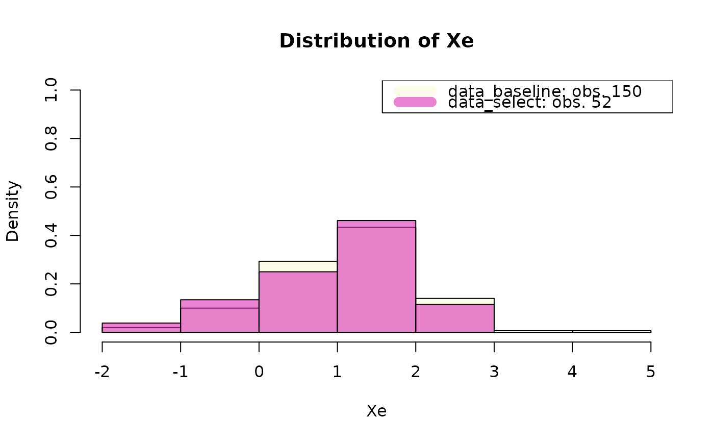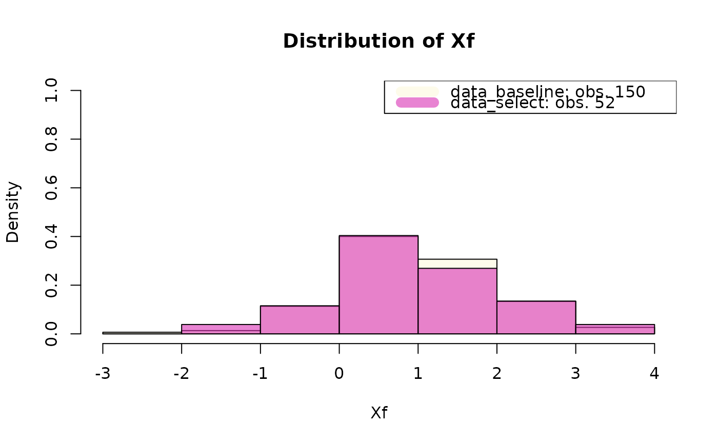
Compare distributions of shared variables across data sets (histograms/barplots)

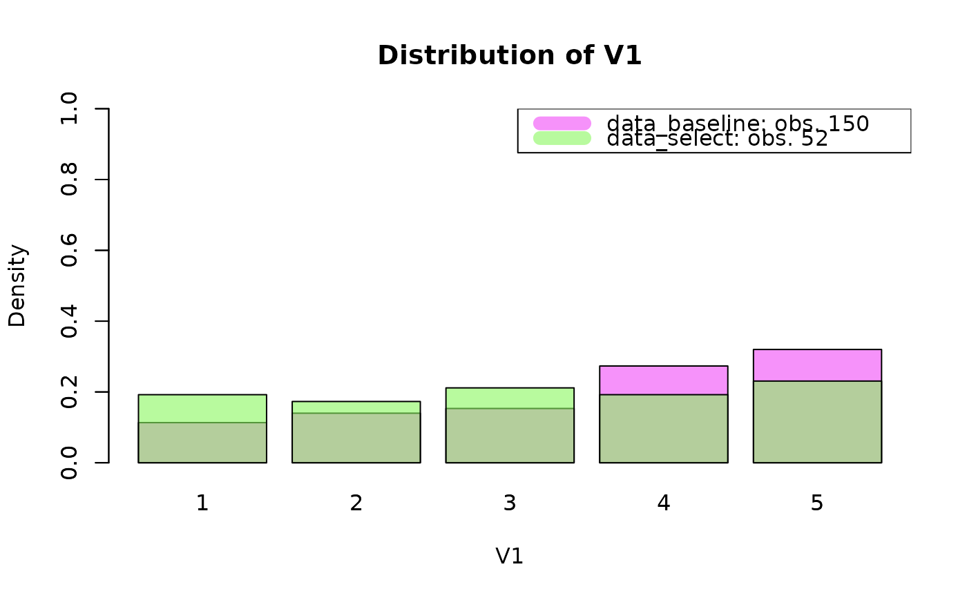
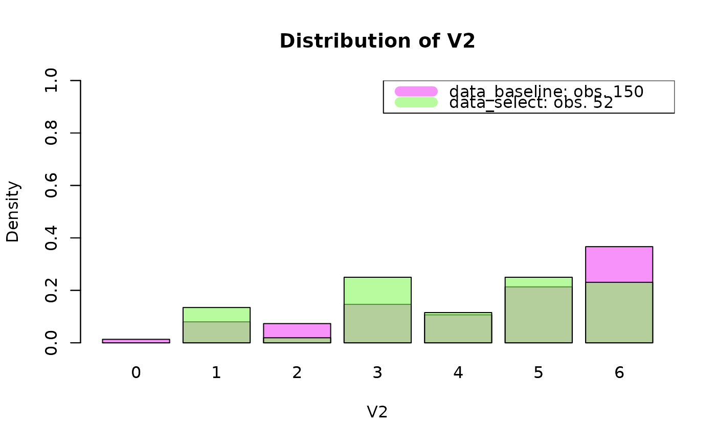
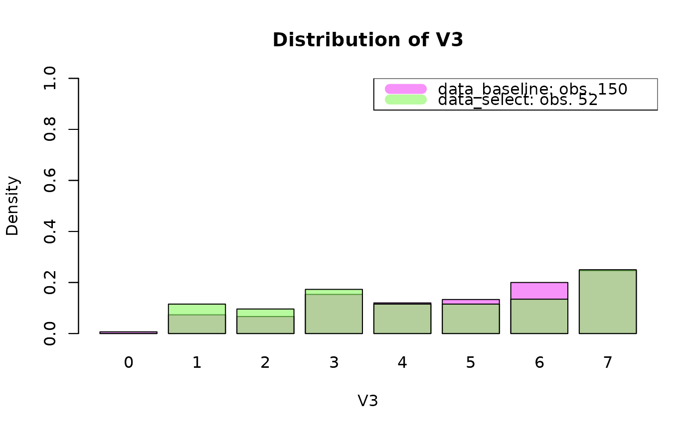
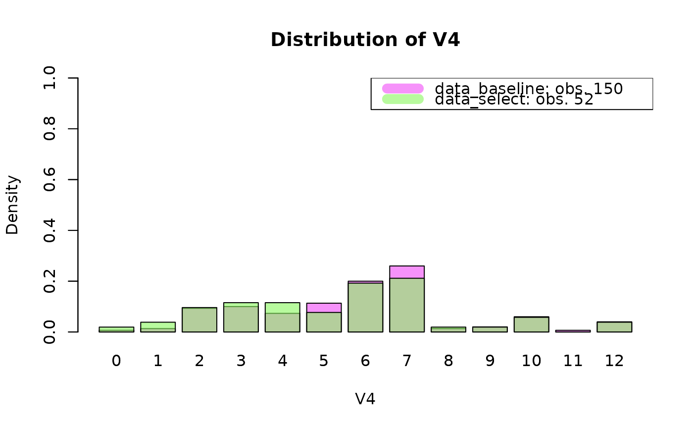
Overlays, for each variable in common_vars, the empirical distribution in every data set of data_list (e.g. a baseline file vs. the linked set).

Usage

plot_distributions(data_list, common_vars, threshold, colours = NULL)

Arguments

data_list: Named list of data frames, each containing common_vars.
common_vars: Character vector, variables to compare.
threshold: Numeric, the linkage decision rule that defined the linked data; only used to label the linked data in the legend.
colours: Optional vector of colours, one per element of data_list.

Value

NULL, invisibly; called for its plotting side effect.

Examples

PIVs_config <- list( V1 = list(dynamics = "stable",
                               bound_mistakes = c(0.10,0.10),
                               fix_mistakes = c(NA,NA)),
                     V2 = list(dynamics = "stable",
                               bound_mistakes = c(0.10,0.10),
                               fix_mistakes = c(NA,NA)),
                     V3 = list(dynamics = "flexible",
                               bound_mistakes = c(NA,NA),
                               fix_mistakes = c(NA,NA)),
                     V4 = list(dynamics = "structured",
                               bound_mistakes = c(NA,NA),
                               fix_mistakes = c(0.03,0.03),
                               cond_hazard_cov = list(cov1=c("Xe", "Xf"),
                                                      cov2=c())) )
n_values  <- c( 5, 6, 7, 12 )
p_mistake <- list( V1 = c(0.02, 0.02), V2 = c(0.02, 0.02),
                   V3 = c(0.05, 0.05), V4 = c(0.02, 0.02) )
p_missing <- list( V1 = c(0.005, 0.005), V2 = c(0.005, 0.005),
                   V3 = c(0.005, 0.005), V4 = c(0.005, 0.005) )
cond_hazard_params <- list( V1 = c(), V2 = c(), 
                             V3 = c(), V4 = log(c(0.7, 0.6, 0.5)) )
gen_data <- simulate_data( PIVs_config, n_values, c(150, 200), 100, 
                           p_mistake, p_missing, cond_hazard_params, TRUE )
prep_data <- prepare_data( gen_data$data1, gen_data$data2, "1", "2",
                           PIVs_config, TRUE, "entity_id", TRUE )
#> Warning: PIVs 'V4' and 'V2' are associated (Cramer's V = 0.31 in data1, 0.28 in data2); FlexRL assumes conditional independence between PIVs, consider merging or dropping one.
#> '2' is the larger source, saved as B; '1' saved as A.
fit <- StEM( data = prep_data, StEM_iter = 10, StEM_burnin = 5,
             gibbs_iter = 10, gibbs_burnin = 5, n_post_sample = 10 )
#> FlexRL
threshold_strict <- stats::quantile(fit$Delta$x, 0.75)
data_list = list(data_baseline = prep_data$encodedA, 
data_select = prep_data$encodedA[fit$Delta[fit$Delta$x > threshold_strict, "i"],])
common_vars = names(PIVs_config)
plot_distributions(data_list, common_vars)




common_vars = c("Xe", "Xf")
plot_distributions(data_list, common_vars)