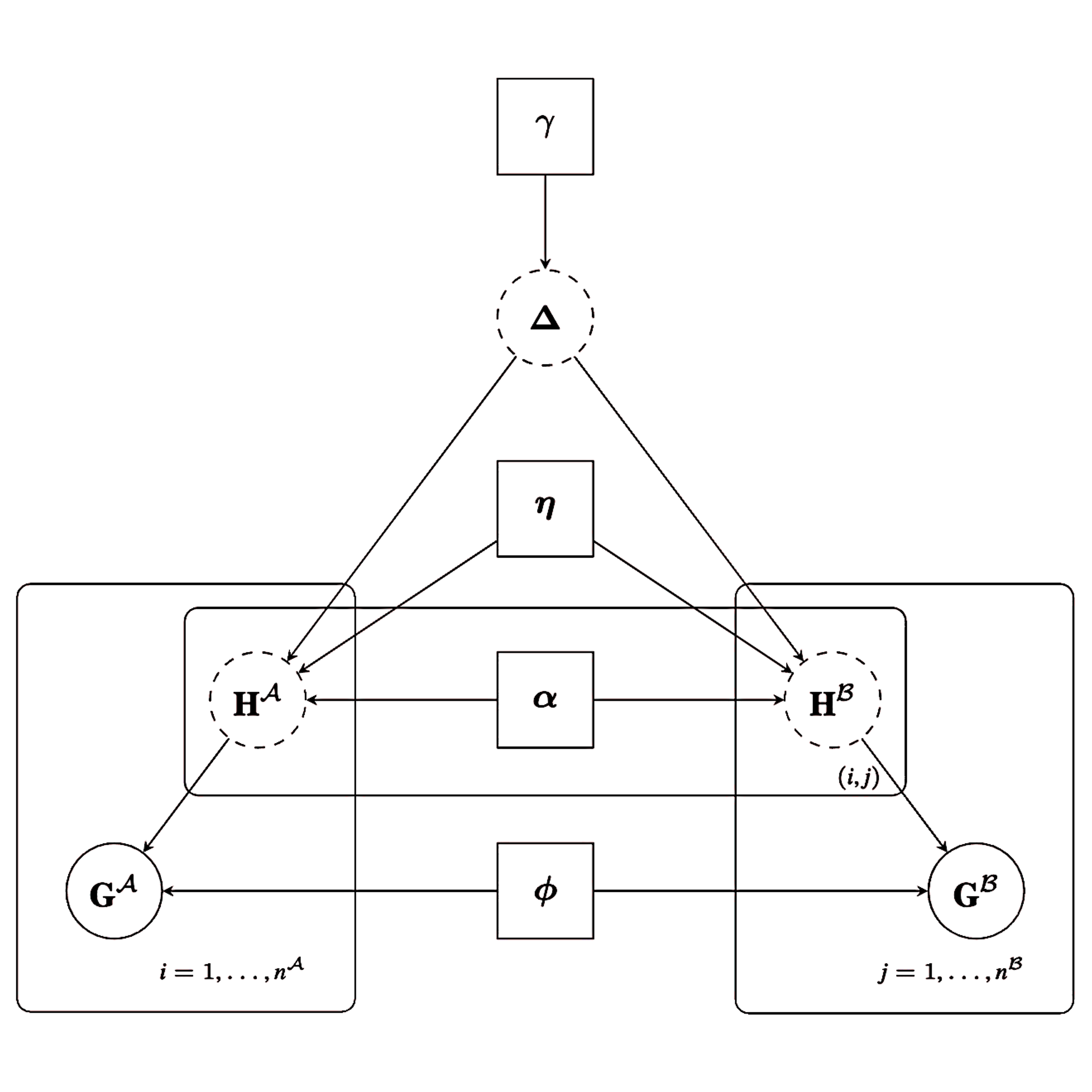
Fits the FlexRL model with a Stochastic EM algorithm: each iteration runs
a Gibbs sampler (alternating between simulating the true PIV values and
the linkage matrix D) and then updates the model parameters (gamma,
eta, alpha, phi) from the post-burn-in Gibbs draws. See the
methodology paper https://10.1093/jrsssc/qlaf016 for details.
Usage
StEM(
  data,
  StEM_iter = 30,
  StEM_burnin = 15,
  gibbs_iter = 20,
  gibbs_burnin = 10,
  music_on = FALSE,
  new_directory = NULL,
  save_info_iter = FALSE,
  gamma0 = NULL,
  phiA0 = NULL,
  phiB0 = NULL,
  n_post_sample = 1000,
  model_dynamics = survival_model("exponential"),
  threads = 1
)
Arguments
- data
List, typically the output of
prepare_data(), with:encodedA(smaller source, PIVs encoded to natural numbers,0= missing),encodedB(larger source, encoded),n_values,same_mistakes(logical: same mistake parameter shared by A and B?),PIVs_config(named list, one entry per PIV, each a list with:dynamics("stable","flexible", or"structured"),bound_mistakes(length-2 numeric/NA, upper bound on the mistake probability in file 1 / file 2),fix_mistakes(length-2 numeric/NA, mistake probability fixed to this value in file 1 / file 2), and, only fordynamics = "structured",cond_hazard_cov(a list withcov1andcov2, the names of covariates in file 1 / file 2 used to model the hazard of change).- StEM_iter
Integer, total number of StEM iterations (including burn-in).
- StEM_burnin
Integer, number of StEM iterations discarded as burn-in.
- gibbs_iter
Integer, total number of Gibbs iterations per StEM step (including burn-in).
- gibbs_burnin
Integer, number of Gibbs iterations discarded as burn-in (
0lets the algorithm auto-detect burn-in from the stabilisation of the linked count).- music_on
Logical; if
TRUE, opens a short tune in the browser when the algorithm finishes.- new_directory
Path to an existing directory to save progress after each iteration, or
NULLto disable.- save_info_iter
Logical; save the environment at the end of each iteration (only used if
new_directoryis notNULL).- gamma0
Optional starting values for
gamma; at random ifNULL.- phiA0
Optional starting values for
phi; at random ifNULL.- phiB0
Optional starting values for
phi; at random ifNULL.- n_post_sample
Integer, number of posterior draws used to estimate the final linkage probabilities
Delta. Default is set to 1000, we recommend not lowering it.- model_dynamics
Object from
survival_model(): the survival model for the change over time of the structured PIVs (default exponential).- threads
Integer, number of OpenMP threads used by the C++ Gibbs kernels for their per-pair loops (default 4). Results are identical for any value. Ignored — the code runs sequentially — if the package was built without OpenMP support.
Value
A list with: Delta sparse-matrix summary (i, j, x) of
posterior linkage probabilities; a pair is a valid link candidate once
x > 0.5 (one-to-one constraint), gamma, eta, alpha, phi the StEM
chains for each parameter.
Examples
PIVs_config <- list( V1 = list(dynamics = "stable",
                               bound_mistakes = c(0.10,0.10),
                               fix_mistakes = c(NA,NA)),
                     V2 = list(dynamics = "stable",
                               bound_mistakes = c(0.10,0.10),
                               fix_mistakes = c(NA,NA)),
                     V3 = list(dynamics = "flexible",
                               bound_mistakes = c(NA,NA),
                               fix_mistakes = c(NA,NA)),
                     V4 = list(dynamics = "structured",
                               bound_mistakes = c(NA,NA),
                               fix_mistakes = c(0.03,0.03),
                               cond_hazard_cov = list(cov1=c("Xe", "Xf"),
                                                      cov2=c())) )
n_values  <- c( 5, 6, 7, 12 )
p_mistake <- list( V1 = c(0.02, 0.02), V2 = c(0.02, 0.02),
                   V3 = c(0.05, 0.05), V4 = c(0.02, 0.02) )
p_missing <- list( V1 = c(0.005, 0.005), V2 = c(0.005, 0.005),
                   V3 = c(0.005, 0.005), V4 = c(0.005, 0.005) )

cond_hazard_params1 <- list( V1 = c(), V2 = c(),
                             V3 = c(), V4 = log(c(0.7, 0.6, 0.5)) )
gen_data <- simulate_data( PIVs_config, n_values, c(150, 200), 100,
                           p_mistake, p_missing, cond_hazard_params1, TRUE )
prep_data <- prepare_data( gen_data$data1, gen_data$data2, "1", "2",
                           PIVs_config, TRUE, "entity_id", TRUE )
#> Warning: PIVs 'V4' and 'V1' are associated (Cramer's V = 0.31 in data1, 0.19 in data2); FlexRL assumes conditional independence between PIVs, consider merging or dropping one.
#> '2' is the larger source, saved as B; '1' saved as A.
fit1 <- StEM( data = prep_data, StEM_iter = 5, StEM_burnin = 2,
              gibbs_iter = 5, gibbs_burnin = 2, n_post_sample = 5,
              model_dynamics = survival_model("exponential") )
#> FlexRL
apply(fit1$alpha$V4[2:5,], 2, mean)
#>   intercept          Xe          Xf
#> -0.08812096 -0.57437484 -0.47599521
cond_hazard_params1$V4
#> [1] -0.3566749 -0.5108256 -0.6931472
head(fit1$Delta[fit1$Delta$x > 0.5, ])
#>    i j   x
#> 1  1 1 1.0
#> 4  4 4 1.0
#> 5  5 5 1.0
#> 6 77 6 0.8
#> 7  7 7 1.0
#> 8  8 8 1.0

cond_hazard_params2 <- list( V1 = c(), V2 = c(),
                             V3 = c(), V4 = log(c(0.3, 0.7, 0.6, 0.5)) )
gen_data <- simulate_data( PIVs_config, n_values, c(150, 200), 100,
                           p_mistake, p_missing, cond_hazard_params2, TRUE,
                           model_dynamics = survival_model("weibull") )
prep_data <- prepare_data( gen_data$data1, gen_data$data2, "1", "2",
                           PIVs_config, TRUE, "entity_id", TRUE )
#> '2' is the larger source, saved as B; '1' saved as A.
fit2 <- StEM( data = prep_data, StEM_iter = 5, StEM_burnin = 2,
              gibbs_iter = 5, gibbs_burnin = 2, n_post_sample = 5,
              model_dynamics = survival_model("weibull"))
#> FlexRL
apply(fit2$alpha$V4[2:5,], 2, mean)
#>   log_shape   intercept          Xe          Xf
#>  0.00925035 -1.18432592  0.14060766 -0.59662506
cond_hazard_params2$V4
#> [1] -1.2039728 -0.3566749 -0.5108256 -0.6931472
head(fit2$Delta[fit2$Delta$x > 0.5, ])
#>      i j   x
#> 4    4 4 0.8
#> 6    5 5 0.6
#> 7    6 6 0.8
#> 9  128 7 0.8
#> 10  61 8 1.0
#> 11   9 9 0.8

cond_hazard_params3 <- list( V1 = c(), V2 = c(),
                             V3 = c(), V4 = log(c(0.3, 0.7, 0.6, 0.5)) )
gen_data <- simulate_data( PIVs_config, n_values, c(150, 200), 100,
                           p_mistake, p_missing, cond_hazard_params3, TRUE,
                           model_dynamics = survival_model("gompertz") )
prep_data <- prepare_data( gen_data$data1, gen_data$data2, "1", "2",
                           PIVs_config, TRUE, "entity_id", TRUE )
#> '2' is the larger source, saved as B; '1' saved as A.
fit3 <- StEM( data = prep_data, StEM_iter = 5, StEM_burnin = 2,
              gibbs_iter = 5, gibbs_burnin = 2, n_post_sample = 5,
              model_dynamics = survival_model("gompertz"))
#> FlexRL
apply(fit3$alpha$V4[2:5,], 2, mean)
#>           g   intercept          Xe          Xf
#> -1.13048839 -2.14282882 -0.08845059  0.39299854
cond_hazard_params3$V4
#> [1] -1.2039728 -0.3566749 -0.5108256 -0.6931472
head(fit3$Delta[fit3$Delta$x > 0.5, ])
#>      i  j   x
#> 3    3  3 1.0
#> 5    6  6 1.0
#> 10 116 11 0.8
#> 11  12 12 1.0
#> 12  13 13 0.8
#> 14  15 15 1.0

cond_hazard_params4 <- list( V1 = c(), V2 = c(),
                             V3 = c(), V4 = log(c(0.6, 0.5, 0.4, 0.3, 0.2, 0.1)) )
gen_data <- simulate_data( PIVs_config, n_values, c(150, 200), 100,
                           p_mistake, p_missing, cond_hazard_params4, TRUE,
                           model_dynamics = survival_model("piecewise", cuts = c(1,2,3)) )
prep_data <- prepare_data( gen_data$data1, gen_data$data2, "1", "2",
                           PIVs_config, TRUE, "entity_id", TRUE )
#> '2' is the larger source, saved as B; '1' saved as A.
fit4 <- StEM( data = prep_data, StEM_iter = 2, StEM_burnin = 1,
              gibbs_iter = 2, gibbs_burnin = 1, n_post_sample = 2,
              model_dynamics = survival_model("piecewise", cuts = c(1,2,3)))
#> FlexRL
#> Warning: PIV 'V1', file A hit its mistake bound on 50% of StEM iterations.
#>   PIV 'V1', file B hit its mistake bound on 50% of StEM iterations.
apply(fit4$alpha$V4, 2, mean)
#>        log_h1        log_h2        log_h3        log_h4            Xe
#>  -0.124675252  -1.965644581 -19.676423339  -1.218537916   0.007940481
#>            Xf
#>  -0.224878671
cond_hazard_params4$V4
#> [1] -0.5108256 -0.6931472 -0.9162907 -1.2039728 -1.6094379 -2.3025851
head(fit4$Delta[fit4$Delta$x > 0.5, ])
#>     i j x
#> 1   1 1 1
#> 2   2 2 1
#> 3 107 3 1
#> 4   4 4 1
#> 5   5 5 1
#> 6   6 6 1